
Part of The AI Infrastructure Reality Check.
In the model below, the GPUs arrive in month 12. The operator can send its first bill in month 25. Move the delivery up four months and the invoice date stays put. Finish the grid work four months early and billing moves up one month. The delivery date on a purchase order tells you when the equipment gets to the site. Billing depends on when the operator has a working cluster the customer can accept.
CoreWeave reported over 4.6 GW of contracted power and over 1.7 GW of active power at the end of September 2026. Look at one lease in its quarterly filing. The company was still waiting for 453 MW and expected that power to arrive in phases. At campus scale, a signature can precede delivery by years. CoreWeave Q3 2026 results · CoreWeave Form 10-Q, Note 8
Work backward from the first customer handoff
The model covers one cluster at one site. The operator can bill once the customer accepts the system under the contract. Before that, the operator has to commission it, which means installing the equipment and checking it under load. The accelerators and network fabric have to be in place, the building needs working cooling and the utility needs to connect the power. The customer must be ready to integrate the cluster by the time acceptance starts.
| Branch | Predecessor | Ready in month |
|---|---|---|
| Financing | Project start | 2 |
| Accelerator delivery | Financing | 12 |
| Network fabric delivery | Financing | 16 |
| Building and cooling | Financing, then permits | 19 |
| Energization | Grid connection and switchgear | 20 |
| Customer readiness | Financing | 18 |
| Commissioning | Energization, cooling, GPUs, and fabric | 23 |
| Contractual acceptance | Commissioning and customer readiness | 25 |
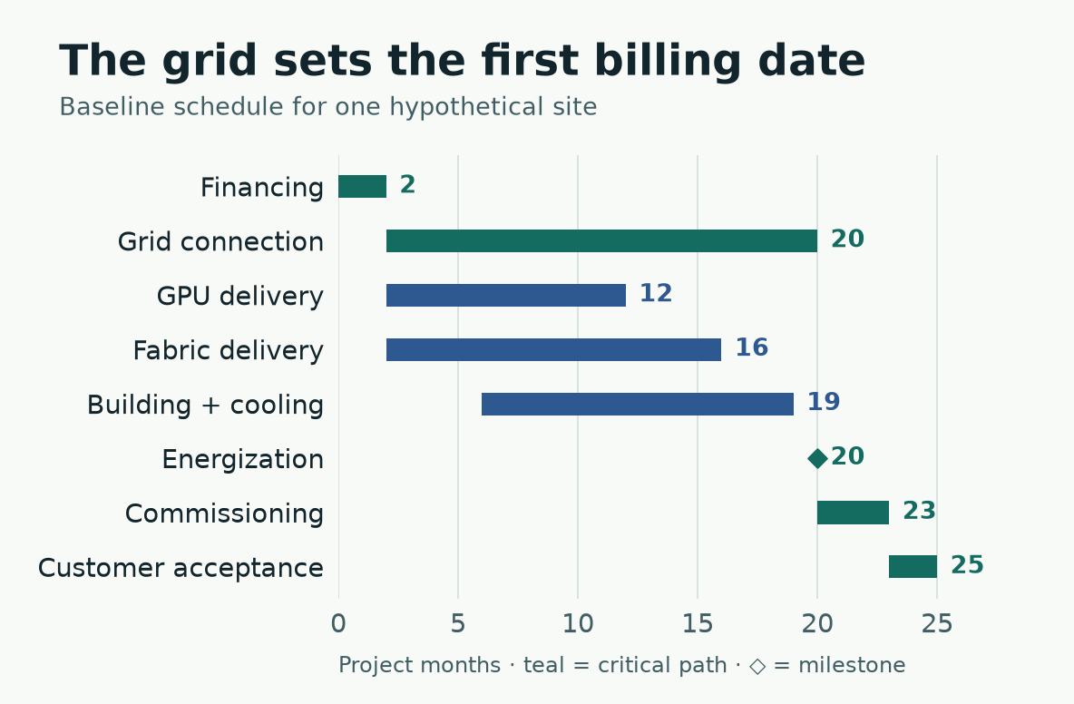
Teal marks the baseline critical path. The chart shows selected tasks, with switchgear and permitting dependencies retained in the model.
Each task waits for its last prerequisite. The switchgear is ready in month 14 and the grid connection in month 20, so the crew can energize the site in month 20. Commissioning takes three months. Acceptance takes two. The grid connection is on the critical path, the chain of work that determines the earliest possible finish. Cooling has one month to slip before it pushes back commissioning. The fabric has four.
An accelerator delivery in month 8 leaves the operator carrying the equipment four months longer, with billing still fixed at month 25. Paying for an earlier shipment may be worth it if it buys protection against a later shortage. Before signing, check whether the supplier can hold the shipment and who pays for storage and financing.
Which deadline moves the billing date?
| Change to the baseline | First billable month | Branch holding up commissioning |
|---|---|---|
| None | 25 | Grid |
| Accelerators arrive four months earlier | 25 | Grid |
| Grid work finishes four months earlier | 24 | Building and cooling |
| Grid work and cooling finish four months earlier | 21 | Grid and fabric, tied |
| Fabric arrives five months later | 26 | Fabric |
If the grid work finishes early, the commissioning crew waits for the building and cooling instead. Shorten both schedules and the grid connection and fabric delivery land in month 16. With those dates tied, billing moves up again only if both jobs finish earlier.
To build this schedule for a specific site, you need dates for the milestones in the table. A connection request gives you an earlier point in the process. In its preliminary November 2026 update, ERCOT counted responses from 433 loads that together requested about 177 GW of interconnection capacity. Some applicants were still deciding what cooling equipment to use. Track how many megawatts make it from request to agreement to energization before putting them in a construction schedule. ERCOT preliminary data center impact survey, November 5, 2026
Move a date in the interactive critical-path simulator, or download the Python model to calculate finish dates and critical paths. Run python3 physical-infrastructure-models.py deployment for the cases above. Add --task grid --months 14 to set the duration of the grid task to 14 months, counted from the end of its prerequisite. The simulator uses fixed dependencies and durations. For a construction budget, allow a range of finish dates. If several jobs share a crew or vendor, account for the chance that they’ll all slip together.
After commissioning, measure every constraint in one unit
Once a new campus has secured its racks, I’d check when it can draw firm power. At a site already serving customers, pick one workload and measure what each part of the system can sustain. Count the requests that finish within its service-level objective (SLO), such as a latency target. Otherwise a change that leaves customers waiting longer can look like a throughput gain. IEA on grids
Suppose the GPUs can handle 72,000 qualifying requests an hour. The site has enough power for 80,000, enough cooling for 100,000 and enough network capacity for 90,000. Customers are asking for 92,000. This exercise gives each resource an independent ceiling for the same workload at a fixed operating point.
| Cumulative change | Accelerator limit | Power | Cooling | Fabric | Demand | Served | Active limit |
|---|---|---|---|---|---|---|---|
| Baseline | 72 | 80 | 100 | 90 | 92 | 72 | Accelerators |
| More accelerators | 120 | 80 | 100 | 90 | 92 | 80 | Power |
| More firm power | 120 | 110 | 100 | 90 | 92 | 90 | Fabric |
| Fabric upgrade | 120 | 110 | 100 | 115 | 92 | 92 | Demand |
| Demand grows | 120 | 110 | 100 | 115 | 105 | 100 | Cooling |
The table gives hypothetical rates in thousands of requests an hour. Add room for 48,000 more requests at the accelerators and the site serves only 8,000 more. Power runs out first. Upgrade power and the fabric, and the site can serve everyone who shows up. More demand brings cooling into play. If demand drops to 70,000, that same site serves 70,000.
Run the measurement again after a change. Adding racks can mean more communication between racks, especially if the team changes how it splits the workload across GPUs. Draw more power and the cooling headroom can shrink as the equipment gets hotter. The model holds those interactions fixed. A purchasing decision needs measurements from the proposed layout.
Run python3 physical-infrastructure-models.py bottlenecks with the downloadable scenario model to reproduce the table. Replace the limits with measurements from your workload before testing an upgrade. When a 50% increase in one resource buys 5% more useful throughput, check which resource tops out next.
During a power cap, the queue can become the limit
The allocation problem looks different when a utility asks a running site to cut its load. In March 2026, Google reported signing 1 GW of demand-response capacity across its U.S. data-center agreements and said it can move some machine-learning work. The Zeus authors tested power caps and batch sizes on several deep-learning training workloads and measured energy-efficiency gains of 15.3% to 75.8%. An inference scheduler still needs to know how a power cap will change latency for the requests it serves. Google demand-response announcement · Zeus, NSDI 2023
In the Python model, twelve rack groups can reserve up to 10 MW. Facility loads and shared services take a fixed 1.6 MW. A rack group at full power reserves 700 kW and serves ten requests a minute. The first capped configuration reserves 450 kW and serves eight requests a minute per group. At 7.2 MW, the scheduler checks every allocation that fits and can pick the one with the highest modeled service rate. It handles requests in arrival order.
Every run gets the same 30 minutes of traffic. The queue receives 75 requests a minute, rising to 100 a minute for a ten-minute burst. A request counts as on time if it finishes within two one-minute slots of arrival, including service. After the 30 minutes, the scheduler keeps running until the queue empties. The power column records the capacity each policy reserves.
| Policy | Reserved MW | Completed/min during arrivals | Service-slot utilization | p95 latency | On time | Peak backlog |
|---|---|---|---|---|---|---|
| 12 full-power groups | 10.0 | 83.3 | 69.4% | 1 min | 100% | 0 |
| 8 full-power groups | 7.2 | 78.3 | 97.9% | 4 min | 54.2% | 200 |
| 12 capped groups | 7.0 | 83.3 | 86.8% | 2 min | 100% | 40 |
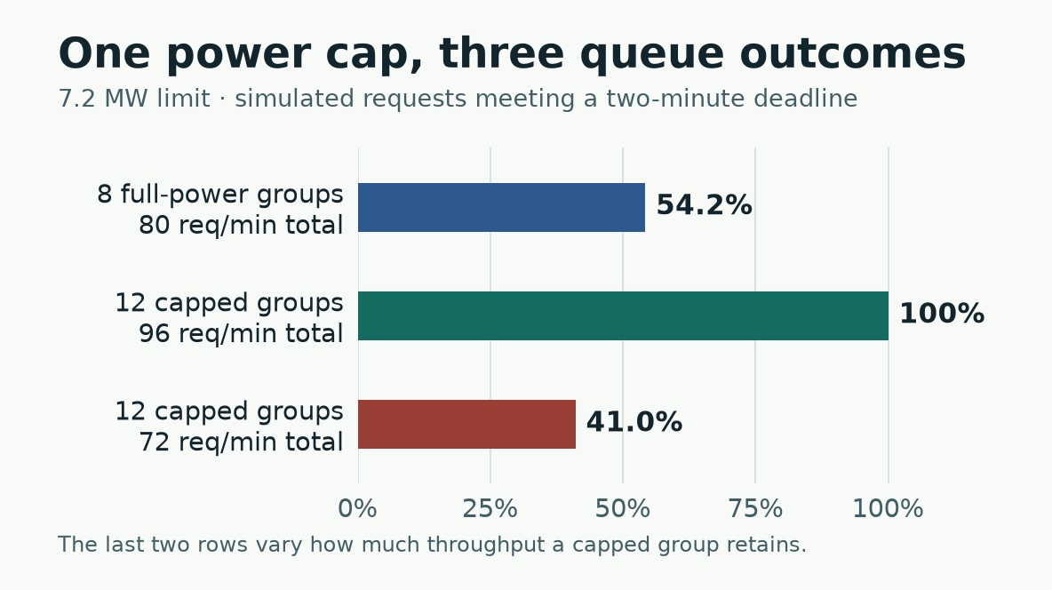
The same arrival trace and power limit apply to all three cases. The last two rows change how much throughput a capped group retains.
At 7.2 MW, eight groups at full power leave 200 requests in the queue at the peak. Twelve groups at reduced power bring the peak to 40. At 450 kW, each capped group in that run keeps 80% of its capacity on about 64% of its full power reservation.
Take the same workload and assume each capped group keeps just 60% of its capacity. The twelve groups then offer 72 slots a minute. The 95th-percentile (p95) latency rises to six minutes and only 41.0% of requests finish on time. Eight full-power groups still deliver a p95 of four minutes and 54.2% on time. The search picks capped groups when they keep more of their capacity and full-power groups when capping costs more throughput. That search maximizes capacity for identical jobs. A scheduler for a mixed fleet has to account for which traffic classes can move.
Run python3 physical-infrastructure-models.py power with the downloadable scheduler, then add --capped-rate 6 to give each capped group six slots per minute. The model treats all requests alike, holds service capacity constant within each slot and fixes the site overhead. For a curtailment drill, replay a burst at each power setting and measure throughput, tail latency and queue drain time. The last delayed request can still be waiting after the site has met its power target.